Whenever a fluid flows through a conduit pressure loss occurs. Many methods are available to calculate frictional pressure losses. They range from simple empirical equations to rigorous mechanistic multiphase flow models.
Darcy-Weisbach flow equation:
The Darcy-Weisbach flow equation is theoretically sound equation derived from the Conservation of Mass and Conservation of Momentum laws. Named after Henry Darcy and Julius Weisbach, it relates the pressure loss due to friction along a given length of pipe to the average velocity of the fluid flow for an incompressible fluid.
The Darcy-Weisbach equation contains a dimensionless friction factor, known as the Darcy friction factor. This is also variously called the Darcy–Weisbach friction factor, friction factor, resistance coefficient, flow coefficient, or Moody friction factor.
In a cylindrical pipe of uniform hydraulic diameter d, flowing full, the pressure loss due to density and viscous effects dp/dL is proportional to length L and can be characterized by the Darcy–Weisbach equation:
![]()
Where:
- dP/dL = Pressure Gradient (psi/ft)
- f = friction factor
- ρ = Fluid density (lb/ft3)
- v = Fluid velocity (ft/s))
- d = Hydraulic diameter (ft))
The equation can be written as shown below in both typical US oilfield units and SI units:
|
Typical US oilfield units
Where: · dP/dL = Pressure Gradient (psi/ft) · f = friction factor · SG = Fluid specific gravity (relative to water) · ν = Fluid velocity (ft/s)) · d = Hydraulic diameter (in) |
SI units
Where: · dP/dL = Pressure gradient (KPa/m) · f = friction factor · SG = Fluid specific gravity (relative to water) · ν = Fluid velocity (m/s) · d = Hydraulic diameter (mm) |
Nota bene: One of the traditionally used formulas to calculate friction losses is the Hazen-Williams equation. It is an empirical formula developed for municipal water distribution systems. It relates the flow of water in a pipe with the physical properties of the pipe and the pressure drop caused by friction. It has the advantage that is not a function of the Reynolds number, but it works reasonably well only when water is the flowing medium and should not be used to calculate friction losses in viscous or gassy fluids.
Friction Factor:
The friction factor fD is not a constant: it depends on such things as:
- The characteristics of the pipe (diameter D and roughness height ε),
- The characteristics of the fluid (especially its kinematic viscosity ν),
- And the velocity of the fluid flow.
It has been measured to high accuracy within certain flow regimes and may be evaluated by the use of various empirical relations, or it may be read from published charts. These charts are often referred to as Moody diagrams, after L. F. Moody, and hence the factor itself is sometimes erroneously called the Moody friction factor.
- Moody diagram:
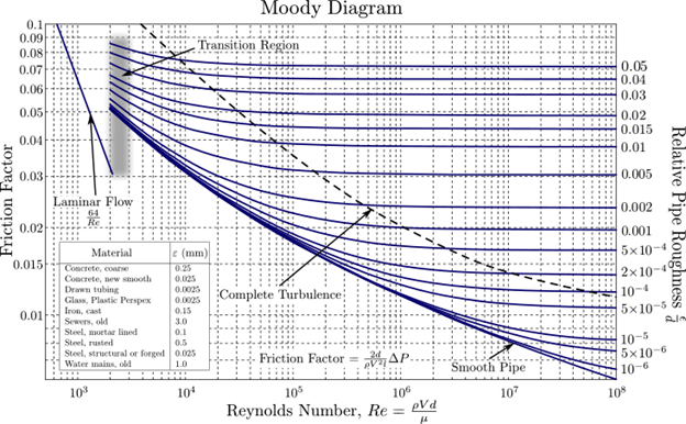
The Moody diagram is a graph in non-dimensional form that relates the Darcy-Weisbach friction factor fD, Reynolds number Re, and relative roughness for fully developed flow in a circular pipe. It can be used for working out pressure drop or flow rate down such a pipe.
The following Figure shows the Moody diagram. The Darcy-Weisbach friction factor fD plotted against Reynolds number Re for various relative roughness ε / D:
- Variation of Friction Factor with Flow Regime:
There are three broad flow regimes of fluid flow: laminar, critical, and turbulent. The friction factor in each flow regime is dependent upon the Reynolds number.
Reynolds number is expressed as below:
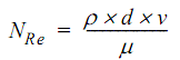
Where:
- NRe = Reynold number
- ρ = Fluid density (lb/ft3 or gm/m3)
- d = Pip diameter (ft or m)
- ν = Fluid velocity (ft/s or m/s)
- μ = Fluid viscosity
In typical US Oilfield units, the Reynold number equation can be written as per the following equation:
![]()
Where:
- NRe = Reynold number
- SG = Fluid specific gravity (relative to water)
- d = Pip diameter (in)
- ν = Fluid velocity (ft/s)
- μ = Fluid viscosity (cP)
Laminar Flow Regime:
For laminar flows, where Reynolds numbers are less than 2100, the fluid is in a smooth flow and the friction factor is calculated directly from Poiseuille’s law:
![]()
Where:
- f = friction factor
- μ = Fluid viscosity
- ρ = Fluid density (lb/ft3 or g/m3)
- d = Pip diameter (ft or m)
- v = Fluid velocity (ft/s or m/s)
- NRe = Reynolds number
Turbulent Flow Regime:
If the Reynolds number is greater than 2100, the fluid is in turbulent flow and friction factor must be looked up in a chart, such as Moody diagram, or calculated from empirical equations. The relationship between the friction factor fD, the Reynolds number Re, and the relative roughness ε / D is more complex and is solved using an iterative calculation. One model for this relationship is the Colebrook equation which is an implicit equation in fD. Colebrook’s Friction Factor equation is depicted below:
![]()
Where:
- f = friction factor
- ε = Absolute pipe roughness (ft or m)
- d = Pip diameter (ft or m)
- NRe = Reynolds number
Highly Turbulent Flow Regime:
For highly turbulent flow, the friction factor can be calculated from Nikuradse’s equation. An iterative calculation is not required to solve this equation. It can be solved directly:
![]()
Where:
- f = Moody friction factor
- ε = Absolute pipe roughness (ft or m)
- d = Pip diameter (ft or m)
While the Darcy-Weisbach equation adjusts friction loss for viscous (Newtonian) fluids, it does not account for two-phase flow as occurs if gas breaks out of solution as in the upper portions of the tubing.
Reference:
- Darcy–Weisbach equation
- Moody chart
- Basic ESP Sizing Manual, GE Oil & Gas – ESP, Inc.