ESP Design – Hand Calculations

This article walks through the suggested nine step procedure for selecting and designing an electric submersible pump. This nine step procedure for ESP design is a basic hand-design of simple water and light crude oil. For more complicated well conditions, such as high GOR, viscous oil, high-temperature wells, etc. a number of computer programs are available to automate this process.

Step 1: Basic Data:

As detailed in the article “Step 1: Basic data ”, step 1 of the nine step design procedure is the most important step because all the others design steps will depend on the basic data selected in this step.

In this example, a high water cut well is considered. This is the simplest type of well for sizing submersible equipment.

• Well Profile:

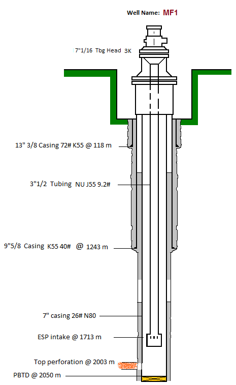
Vertical Well

Casing: 7” 26#

Tubing: 3 ½” 9,2# N80 NU

Top perforation: 2003m

Pump Intake depth: 1713m

• Fluid properties and well conditions:

PVT data non-available

Oil Gravity: 35 API

Water Cut: 90%

Water Gravity: 1,01 rel-H2O

Gas Gravity: 0,8 rel-air

Producing GOR: 200 scf/stb

Bubble Pressure: 964 psi

Bottomhole Temperature: 90 °C

Wellhead Temperature: 50 °C

Wellhead Pressure: 87 psi

Casing-Head Pressure: 15 psi

• Inflow performance:

Present production rate: 2500 bfpd @ Pump Intake Pressure = 1160 psi

Reservoir Pressure: 2320.6 psi

Datum point: 2003m (top perforation).

Pump Intake Pressure: 1160 psi

Desired production rate: 3500 bfpd.

• Power sources:

Available primary voltage: 418 V

Desired frequency range: 40Hz – 65Hz

• Possible problems?

No sand production, no scale deposit

No gas impurities (N2, H2S and Co2).

MF1 experienced frequent starts and stops.

Step 2: Production Capacity:

The theory behind the production capacity calculations was detailed in the post ” ESP design – Step 2: Production Capacity “. It consists on predicting the well inflow performance.

The pump intake pressure (1160 psi) is greater than bubble point pressure (964 psi). So that, the Productivity Index (PI) inflow performance method will most probably give satisfactory results.

PI=Q/(Pr-Pwf)

Firstly, we need to calculate the flowing bottomhole pressure (Pwf). Pwf is calculated from the pump intake pressure (PIP), hydrostatic pressure and friction loss in the casing annulus between the pump setting depth and the datum point. In the given example, as the pump is set 290m above the perforations, the friction loss, because of flow of fluid through the annulus from perforations to pump setting depth, is small, as compared to the flowing pressure, and can be neglected.

Pwf is calculated from the pump intake pressure (PIP), hydrostatic pressure and friction loss in the casing annulus between the pump setting depth and the datum point. In the given example, as the pump is set 290m above the perforations, the friction loss, because of flow of fluid through the annulus from perforations to pump setting depth, is small, as compared to the flowing pressure, and can be neglected.

Therefore:

Pwf = PIP + hydrostatic pressure from pump intake depth to the datum.

Pwf = PIP + 0.433×SG×(2003-1703)×3.28

Because there is both water and oil in the produced fluids, it is necessary to calculate a composite SG of the produced fluids. SG is calculated from oil SG and water SG.

SG(oil) = 141.5 / (°API+131.5) = 141.5 / (35+131.5) = 0.845.

SG(oil) = 0.845

Water Gravity = 1.01.

WC= 90%

SG= 0.9×1.01+(1-0.9)×0.845= 0.9935

SG = 0.9935

Therefore, Pwf= 1160+0.433×0.9935×(2003-1703)×3.28= 1569.8 psi

Pwf = 1569.8 psi.

Thus, PI = 2500/(2320.6-1563.8)=3.33 bpd/psi.

PI = 3.33 bpd/psi.

Let’s calculate, the Pwf at the desired production rate:

From the Productivity Index equation, Pwf = Pr – Q/PI = 2320.6 – 3500/3.33 = 1269.5 psi.

Pwf = 1269.5 psi

And PIP = 1269.5 – (1569.8-1160) = 860 psi.

PIP = 860 psi.

At a liquid rate of 3500 bfpd, the PIP is a bit smaller than the bubble point pressure (964 psi). Therefore, the Productivity Index (PI) inflow performance method will most probably give satisfactory results.

Step 3: Gas Calculations:

It is essential to determine the percentage of free gas by volume at the pumping conditions in order to select the proper pump and gas handling device (if required). All equations used in this section were detailed in the post “ESP design – Step 3: Gas Calculations”.

In this third step, one must determine The total fluid volume (Vt) of oil, water, and gas at the pump intake. For this example, Standing’s correlation was used (Standing is the oldest, simplest and most commonly used correlation).

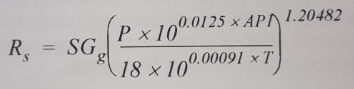
Solution GOR calculation:

Where:

Rs: Solution gas-oil ratio (scf/stb)
API: Oil API gravity
SGg: Gas specific gravity (relative to air)
P: Pressure (psia)
T: Temperature (°F)

To determine the solution GOR (R_s) at the pump-intake pressure, we need to substitute the pump-intake pressure for the pressure (P) in Standing’s equation. For this example, motor temperature is 70 °C (158 °F).

Rs = 0.8 × [ (860 × 10^(0.0125×35)) / (18 × 10^(0.00091 × 158) ]^1.20482

Rs = 190.3 scf/stb

Oil Formation Volume Factor (Bo):

The oil formation volume factor is defined as the ratio of the volume of oil (plus the gas in solution) at any specified temperature and pressure to the volume of oil at standard conditions.

Using the following Standing’s equation, determine the oil formation volume factor (B_o):

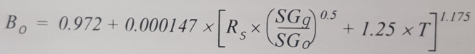
Bo = 0.972 + 0.000147 × [190.3 × (0.8/0.845)^0.5 + 1.25 × 158]^1.175

Bo = 1.131 bbl/stb @ 860 psi pump intake pressure.

Gas Formation Volume Factor (B_g):

Bg the volume, in barrels, that one thousand Standard. cubic feet of gas would occupy at some specific pressure and temperature. It indicates how much the gas volumetrically compresses when taken from Standard conditions (60 ºF, 1 atm) to any other specific conditions.

By assuming 0.85 Z factor, Determine the gas volume factor (B_g):

Bg = 5.05 × 0.85 × (158 + 460) ] / (860)

Bg = 3.085 bbl/Mscf @ 860 psi pump intake pressure.

Now, these three variables: Rs, Bo, and Bg are known. So that, the volumes of oil, water, and free gas can be determined and percentages of each calculated.

Total Gas Volume:

The total volume of gas (both free and in solution) can be determined as:

Total Gas Volume = (producing GOR x Oil rate)

[Oil rate]: stock tank barrels per day.

Total Gas = 200 × 3500 × (1-0.9) = 70000 scf = 70 Mscf

Total Gas Volume = 70 Mscf

Solution Gas Volume:

Using the solution GOR (Rs) at the pump intake, determine the solution gas volume:

Solution Gas Volume = (Solution GOR @ PIP x Oil rate) = (Rs x Oil rate)

Solution Gas Volume = 190.3 × 3500 × (1-0.9) = 66710 scf = 66.71 Mscf

Solution Gas Volume = 66.71 Mscf

Free Gas Volume:

The free gas equals the total gas minus the solution gas. The difference represents the volume of free gas released from solution by the decrease in pressure from bubble point pressure of 964 psi to the pump-intake pressure of 860 psi.

Free Gas Volume = Total Gas Volume – Solution Gas Volume

Free Gas Volume = 70 – 66.7 = 3.29 Mscf

Free Gas Volume = 3.29 Mscf

Volume of oil at the pump intake (Vo):

The volume of oil at the pump intake (Vo) equals stock tank barrels times oil formation volume factor (Bo):

Vo = Bo × BOPD

Vo = 1.131 × 3500 × (1-0.9)= 395.9 bopd

Vo = 395.9 bopd

Volume of gas (Vg) at the pump intake:

The volume of gas (Vg) at the pump intake equals the amount of free gas times gas volume factor (Bg):

Vg = Free Gas x Bg

Vg = 3.29 × 3.085 = 10.15 bgpd

Vg = 10.15 bgpd

Volume of water (Vw) at the pump intake:

The volume of water (Vw) at the pump intake is the same as stock tank barrels:

Vw = Total fluid volume x Water Cut

Vw = 3500 × 0.9 = 3150 bwpd

Vw = 3150 bwpd

Total fluid volume (Vt) of oil, water, and gas at the pump intake:

The total fluid volume (Vt) of oil, water and gas at the pump intake:

Vt = Vo + Vg + Vw

Vt = 395.9 + 10.15 + 3150 = 3556,1 bfpd

Vt = 3556,1 bfpd

Percentage of free gas to total volume of fluids at the pump intake:

The percentage of free gas to total volume of fluids at the pump intake can now be calculated:

% Free Gas = (Vg / Vt) × 100

% Free Gas = (10.15/3556.1) × 100 = 0.29%

% Free Gas = 0.29%

This is a negligible amount of gas, it is expected that pump performance will not be affected by gas, so no need for a gas separator (for more details, refer to the post: ” ESP: Pump Intake “).

Composite Specific Gravity (SG)comp:

To determine the composite specific gravity (SG)comp, the total mass of produced fluid (including gas) needs to be calculated:

The Total Mass of Produced Fluid (TMPF) is:

TMPF = [(BOPD × SGo) + (BWPD × SGw)] × 5.6146 × 62.4 + (GOR × BOPD × SGg × 0.0752)

TMPF = [3500 × (1-0.9) × 0.845) + (3500 × 0.9 × 1.01)] × 5.6146 × 62.4 + (200 × 3500 × (1-0.9) × 0.8 × 0.0752)

TMPF = 1222469,4 lbm/d

The composite specific gravity (SG)comp is:

SGcomp = TMPF /(BFPD × 5.6146 ×62.4)

SGcomp = 1222469,4 / (3500 × 5.6146 ×62.4)

SGcomp = 0.997

Now, we know the total volume of fluid entering the first pump stage (3556,1 bfpd) as well as the composite SG (0.997). we can continue to the next step of the ESP system design.

Step 4: Total Dynamic Head (TDH):

As detailed in the article “Step 4: Total Dynamic Head”, the total pump head refers to feet (meters) of liquid being pumped. TDH is calculated to be the sum of: net well lift (the net vertical distance fluid must be lifted from an operating fluid level in the well), H_L; well-tubing friction loss, F_t; and wellhead pressure head, H_wh.

TDH = H_L + F_t + H_wh  

Net Well Lift Calculation:

H_L = Pump Depth – PIP (ft)

PIP( ft) = PIP / (0.433 psi/ft × SGcomp)

PIP (ft) = 860 / (0.433 × 0.997) = 3209.62 ft

NB: Giuseppe’s comment on this article, is to be considered for the subsequent calculation steps below.

H_L = Pump Depth – PIP (ft) = 5620.08- 3209.84 = 2410.24 ft

H_L = 2859.68 ft

Tubing Friction Loss Calculation (Ft):

Many methods are available to calculate frictional pressure losses. They range from simple empirical equations to rigorous mechanistic multiphase flow models.

The ESP industry has traditionally used the Hazen-Williams formula to calculate these friction losses (in terms of head, not pressure).

The Hazen-Williams formula is an empirical equation developed for municipal water distribution systems. It works reasonably well when water is the flowing medium. However, it should not be used to calculate friction losses in viscous or gassy fluids.

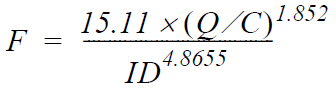
Hazen-Williams Equation:

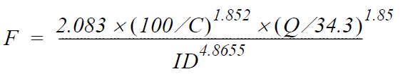
• F = Friction loss factor (ft/1000ft)
• C = Correction Factor (100 for old pipe, 140 for new pipe, 120 for a typical value)
• Q = Volumetric flow rate (bbl/d)
• ID = Pipe inner diameter (in)

This can be simplified to the following equation:

C = 120

Q = 3556,1 bfpd

ID = 2.992″ (tubing: 3 ½” 9,2# N80)

Pump intake depth = 5620.1 ft (1713m)

F = [15.11 × (Q / C)^1.852] / (ID^4.8655)

F= 38.83 ft /1000ft

Therefore, Ft = 38.83 × (5620.1/1000) = 218.26 ft

Ft = 218.26 ft

Wellhead Pressure Head (H_wh):

From the input data, the desired wellhead pressure is 87 psi. Calcultate the corresponding  head at wellhead using the composite SG:

H_wh ( ft) = WHP / (0.433 psi/ft × SGcomp)

H_wh ( ft) = 87 / (0.433 × 0.997)

H_wh ( ft) = 279.26 ft

Total Dunamic Head (TDH) Calculation:

TDH = H_L + F_t + H_wh  

TDH = 2859.68 + 218.26 + 279.26 = 3357.19 ft

TDH = 3357.19 ft

NB: The TDH required is based on normal pumping conditions. If the well is killed with a heavier-gravity fluid, a higher head is required to pump the fluid out, until the well is stabilized on its normal production. Therefore, more horsepower is required to lift the heavier kill fluid. This should be considered when selecting the motor rating for the application.

Step 5: Pump Type:

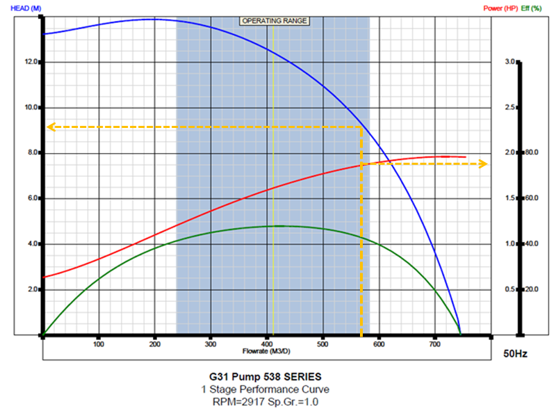
From the manufacturer’s catalog information, select the pump type which will be operating within the recommended operating range and with the highest efficiency at the calculated capacity 3556 bfpd (565 m³/d). The expected production profile of the well has to be covered by the operating range of the pump during the expected ESP run life.

Obviously, the pump ID (series) must fit the 7” 26# casing (ID = 7.276″).

Select the 538 series G31 pump.

NB: When two or more pump types have similar efficiencies at the desired production rate,  refer to the post titled “ESP design – Step 5: Pump Type” to get recommendations on the most adaptable pump to be considered.

Total number of stages required:

From the selected pump performance curve, The head in meters for one stage at 565 m³/d (3556 bfpd) is 8.6 m (28.2 ft). The BHP per stage is 1.875 hp.

To determine the total number of stages required, divide the TDH by the head/stage:

Total number of stages required = TDH/ ( head/stage )

Total number of stages required = (3357.19 /28.1) = 120 stages.

Stages required = 120 stages.

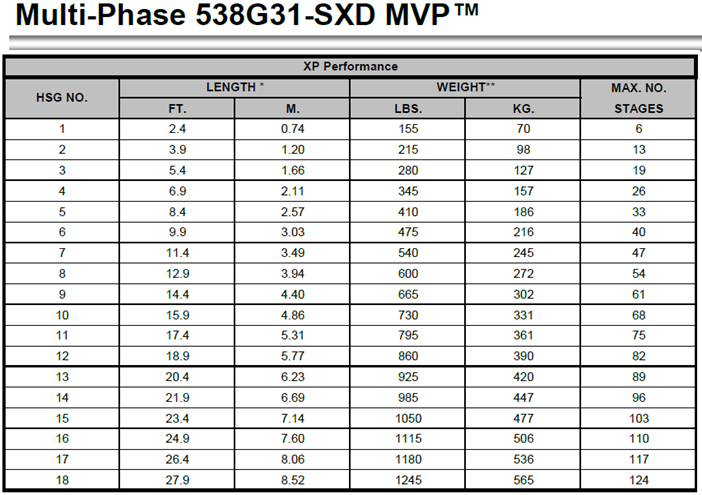
From manufacturer’s information for the Series 538 G31 pump. The housing no. 17 can house a maximum of 117 stages, 124 stages for a housing no. 18.

Either housing no. 17 or 18 should be adequate. In our case, housing no. 18 is selected.

Pump BHP required:

Once the required number of pump stages is decided, calculate the Pump BHP required:

Pump BHP required = BHP/stage × number of stages × SGcomp

Pump BHP required = 1.875 × 124 × 0.997 = 231.8 hp

Pump BHP required = 231.8 hp

Step 6: Optimum Size of Compounds:

The theory behind this step was detailed in the post “ESP design – Step 6: Optimum Size of Compounds”. Actually, ESP downhole compounds have different sizes and can be assembled in a variety of combinations. These combinations must be carefully selected to operate the ESP within production requirement, downhole conditions, material strength, and temperature limits, etc.

Gas Separator / Gas Handler:

As calculated in the “Step 3: Gas Calculations” in this post, the percentage of free gas was negligible (0.29% of the total volume of fluids at the pump intake). So that, no need for a gas separator.

Seal:

It is preferable to select a Seal series the same as that of the pump and the motor. Otherwise, an adaptor is required to connect the units together.

From the manufacturer’s catalog, the 513 series GSB3 DB HL (double-bag, high load thrust bearing) [3 chambers, Bag/Bag/Labyrinth] seal section is selected for this well MF1.

• Seal HP required:

The HP required for the seal depends on the TDH produced by the pump and has to be added to the HP required for the pump. The following Horsepower vs. TDH curve shows a requirement of 2.95 hp for the 513 Series seal operating against a TDH of 3357.19 ft.

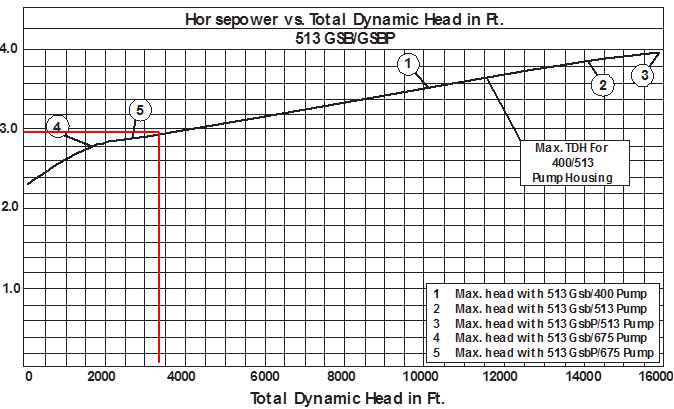
Therefore:

Total HP requirement  = Pump BHP requirement + Seal HP requirement

Total HP requirement  = 231.8 + 2.95

Total HP requirement  = 234.75 hp

• Motor:

When selecting a motor, consideration should be given to choosing as large motor as possible for the casing to optimize the initial cost, motor efficiency, operating cost and ensure better motor cooling (higher fluid velocity).

As mentioned in Step 1: Input Data, MF1 experienced frequent starts and stops. This is why, from the manufacturer’s catalog, we selected an XP motor which is suggested for wells with frequent starts and stops. Select the 333-hp 562 Series motor from the catalog.

The motor voltage can be selected on the basis of considerations discussed in the post “ESP design – Step 6: Optimum Size of Compounds”. For this example, (333 hp; 2321 V; 88 amps) seems to be a good choice.

Check the manufacturer’s catalog and equipment information to assure that all operating parameters are well within their recommended ranges (e.g. shaft HP, housing burst pressure, and fluid velocity).

Typically, the motor is selected to operate in the range from 70 to 100% of its rating. Generally speaking, the maximum motor load should not exceed 110%, in the other hand selecting a motor with minimum operating load (e.g. 10% or 20%) nullifies the protection monitoring of the motor.

Step 7: Optimum Size of Compounds:

As discussed in the previous post: “ESP design – Step 7: Electric Cables”, Cable selection involves the determination of Cable Size, Type and Length.

Determine Cable Size:

• Available space between tubing collars and casing:

Refer to the manufacturer’s cable catalog to determine if the size selected can be used within the proposed tubing and casing sizes. Cable diameter plus tubing-collar diameter will need to be less than the inside diameter of the casing. In our case, all cable sizes can be used.

• Conductor voltage drop calculation:

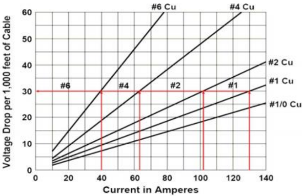
The cable size is selected based on its current carrying capability. Using the motor amps (88) and the following cable voltage drop chart, select a cable size with a voltage drop of less than 30 volts per 1,000 ft.

Conductor sizes #1 and #2 fall in this category. Cables #1 and #2 have voltage drop of 26 volts/1,000 ft and 20 volt/1000 ft @ 25°C (77°F) respectively. Calculate their voltage drop at the downhole temperature (158°F in our case).

For cables operating at a different temperature, the voltage drop can be determined by multiplying it by Temperature Correction Factor (TCF) as indicated in the formula below or by using the table below:
TCF = 1 + 0.00214 × (T – 77)

TCF = 1 + 0.00214 × (158 – 77)= 1.173

Therefore:

cable #1 onductor voltage drop @ (T=158°F) =  20 × 1.173 = 23.46 volts/1,000 ft

cable #2 onductor voltage drop @ (T=158°F) =  26 × 1.173 = 30.5 volts/1,000 ft

• Operating cost comparison: 

I=88A, kWh = 0,05€, cable length= 5720 ft
Size AWG	Resistance (ohm/1000 ft)	Power losses (kW)	Cost of power loss (€/month)	Cost of power loss (€/year)
1	0,139	18,47	665	7980
2	0,17	22,59	813	9759
4	0,271	36,01	1296	15557
6	0,431	57,27	2062	24743

The cable #1 is selected for this well.

Cable Type:

As per the input data, the downhole conditions of this well aren’t considered severe (no risk of corrosion, no sour gases, downhole temperature not high..). So that a standard cable type is selected (with galvanized steel armor).

Refer to the manufacturer’s catalog for more details.

Cable Length:

The pump setting depth is 5620 ft (1713 m). With 100 ft (30.5 m) of cable for surface connections, the total cable length should be 5720 ft (1743.5 m).

Step 8: Optimum Size of Compounds:

As discussed in the previous post: “Step 8 – Downhole and Surface Accessory Equipment”  the required downhole and surface accessory equipment are described in this step 8.

Downhole Accessory Equipment:

• Motor Lead Extension (MLE):

Calculate the length for the MLE:

Pump length = 27.9 ft (8.52 m);

Seal length = 6.3 ft (1.92 m);

Plus 6 ft = 6.0 ft (1.83 m)

= 40.2 ft (12.27 m);

select a standard length of 50 ft (15.24 m) flat cable (AWG: 2, Armor:  Galv.).

• Cable Bands:

Install three bands per section from the motor pothead to the first splice in the power cable (don’t install bands on a cable splice). Place a band above and below the splice approximately 4 inches.

The minimum banding recommendation is two bands per tubing joint, with one band in the middle of the joint and the other band 2 to 3 ft above the collar.

Cross-Coupling Cable Protectors:

Cross-Coupling Cable Protectors are used to protect and support ESP cable. Install a cross-coupling protector every 10 joints.

• Check Valve and drain valve:

Select these accessories on the basis of required ODs and type of threads.

Surface Accessory Equipment:

• Variable Frequency Drive (VFD):

The motor-controller selection is based on its voltage, amperage, and KVA rating. Therefore, before selecting the controller, one must first determine the motor controller voltage.

The surface voltage (SV) is the sum of the motor voltage and the total voltage loss in the cable. Taps on the transformer have to be adjusted to closely achieve this value.

Surface Voltage = Motor Voltage + Conductor Voltage Drop

Surface Voltage = 2321 + [(23.46 Volt/1000 ft × 5720 ft)] = 2455 V.

Surface Voltage = 2455 V.

NB: Surface voltage is less than standard 3 KV cable. 3 kV or higher cable construction can be selected. For this example, a 4 kV power cable is selected.

The motor amperage is 88 amps; the KVA can now be calculated.

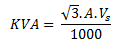Where:

Vs is the required surface voltage, volts.

A is the motor nameplate current, amps.

KVA = (1.73 × 88 × 2455) / 1000 = 374 KVA

KVA = 374

The 380V motor controller: model: 4500-VT (411 KVA / 624 A) suits these requirements.

• Transformers:

The transformer selection is based on the available primary power supply (418 V), the secondary voltage requirement (2455 V) and the KVA requirement (374 KVA).

The 452 KVA Step-Up transformer (C86554) suits these requirements.

• Surface cable:

Select 50 ft (15.2 m) of no. 1 cable for surface connection to transformers.

Step 9: Variable Speed Submersible Pumping System:

As discussed in the previous post: “Step 9 – Variable Speed Submersible Pumping System”,  the most important benefit of using a VSD is the wide flexibility of the variable frequency ESP system. This permits perfect matching of the lift capacity of the ESP system and the well’s productivity. Therefore, it operates over a much broader range of capacity, head, and efficiency.

Since a submersible pump motor is an induction motor, its speed is proportional to the frequency of the electrical power supply. This relationship between variables involved in pump performance (such as head, flow rate, shaft speed) and power is known as “Affinity Laws” (also called “Pump Laws”).

According to the affinity laws, the following relationships exist between the actual speed of the centrifugal pump and its most important performance parameters:

• The flow rate of a pump changes directly proportional to its operating speed.
• The head developed by the pump changes proportionally to the square of the speed.
• The brake horsepower required to drive the pump changes proportionally to the cube of the speed.
• The efficiency of the pump does not change with speed changes.